Tutorial 1: Built in demonstration scripts

# import dlim packages
from dlim.model import DLIM
from dlim.dataset import Data_model
from dlim.api import DLIM_API


import pandas as pd
import matplotlib.pyplot as plt
from scipy.stats import pearsonr
from numpy.random import choice

Load data and split the data into training and validation

Load data, data needs to be a csv file

• the first n-1 columns n-1 genes or different variable, in each genes, there will be multiple mutations

• the last column is fitness value

df_data = pd.read_csv("./data/data_epis_1.csv", sep = ',', header = None)

Load data into tensor format and feed to DLIM later on

Manually split data into 70% for training and 30% for testing

data = Data_model(data=df_data, n_variables=2)
train_id = choice(range(data.data.shape[0]), int(data.data.shape[0]*0.7), replace=False)
val_id = [i for i in range(data.data.shape[0]) if i not in train_id]
train_data = data.subset(train_id)
val_data = data.subset(val_id)

Construct your model and train your data

DLIM model: - n_variables: the number of variables (e.g., genes, environments) - hid_dim: the number of neurons in hidden layers - nb_layer: the number of hidden layers of your NN

DLIM_API:

this is the api to train, predict and plot the final landscape obtained

• model: DLIM model

• flag_spectral: bool, True if use spectral initialization; False, use Xavier-Glorot initialization

• dlim_regressor.fit: train the model with training data

Hyperparameters

• lr: learning rate

• nb_epoch: number of epoches

• batch_size: size of batch

• emb_regularization: weight on regularization on embeddings

• save_path: path for saveing model, if None, the model won’t be saved

model = DLIM(n_variables = train_data.nb_val, hid_dim = 32, nb_layer = 1)
dlim_regressor = DLIM_API(model=model, flag_spectral=True)
losses = dlim_regressor.fit(train_data, lr = 1e-3, nb_epoch=40, batch_size=32, emb_regularization=0, \
                            save_path= './pretrain/harry_epis_model.pt')

spectral gap = 0.865142822265625
spectral gap = 0.568690836429596
Model saved to ./pretrain/harry_epis_model.pt

Show the learning loss during training

plt.figure
plt.plot(losses)
plt.show()

Prediction on validation data

dlim_regressor.predict

• data should be tensor

• detach: bool, True to get numpy array type output; False, get tensor type output

fit_a, var_a, lat_a = dlim_regressor.predict(val_data.data[:,:-1], detach=True)

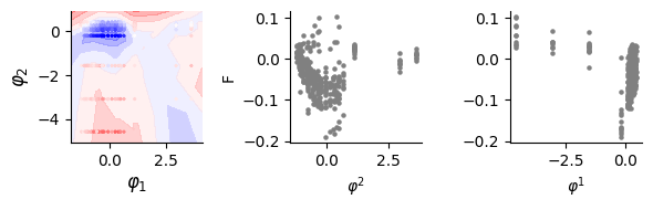
Visualization on landscape

• first panel: landscape by DLIM and dots are measurements

• second panel: the infered phenotype of each mutations on gene 1 versus all fitness mesured on this mutation

• third panel: the infered phenotype of each mutations on gene 2 versus all fitness mesured on this mutation

score = pearsonr(fit_a.flatten(), val_data.data[:, [-1]].flatten())[0]
print(score)

fig, (bx, cx, dx) = plt.subplots(1, 3, figsize=(6, 2))
dlim_regressor.plot(bx, data)

for xx in [bx, cx, dx]:
    for el in ["top", "right"]:
        xx.spines[el].set_visible(False)

# Plot the a00verage curve
print(pearsonr(lat_a[:, 0], val_data[:, -1]))
cx.scatter(lat_a[:, 0], val_data[:, -1], s=5, c="grey")
dx.scatter(lat_a[:, 1], val_data[:, -1], s=5, c="grey")
cx.set_ylabel("F")
cx.set_xlabel("$\\varphi^1$")
dx.set_xlabel("$\\varphi^2$")
plt.tight_layout()
plt.show()

0.9723149104776725
PearsonRResult(statistic=-0.010524778629337813, pvalue=0.8407427503016924)

Use pretrained model

DLIM model: - n_variables: the number of variables (e.g., genes, environments) - hid_dim: the number of neurons in hidden layers - nb_layer: the number of hidden layers of your NN

DLIM_API:

if the model is already saved, you can load the model by add

• load_model: the path of the saved model

• flag_spectral: bool, True if use spectral initialization; False, use Xavier-Glorot initialization

• dlim_regressor.predict: use saved model to predict data

model = DLIM(n_variables = data.nb_val, hid_dim = 32, nb_layer = 0)
dlim_regressor = DLIM_API(model=model, flag_spectral=True, load_model='./pretrain/harry_epis_model.pt')
fit_a, var_a, lat_a = dlim_regressor.predict(data.data[:,:-1], detach=True)

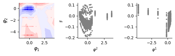
Visualization of obtained landscape

score = pearsonr(fit_a.flatten(), data.data[:, [-1]].flatten())[0]
print(score)

fig, (bx, cx, dx) = plt.subplots(1, 3, figsize=(6, 2))
dlim_regressor.plot(bx, data)

for xx in [bx, cx, dx]:
    for el in ["top", "right"]:
        xx.spines[el].set_visible(False)

# Plot the a00verage curve
print(pearsonr(lat_a[:, 0], data[:, -1]))
cx.scatter(lat_a[:, 0], data[:, -1], s=5, c="grey")
dx.scatter(lat_a[:, 1], data[:, -1], s=5, c="grey")
cx.set_ylabel("F")
dx.set_xlabel("$\\varphi^1$")
cx.set_xlabel("$\\varphi^2$")
plt.tight_layout()
plt.show()

0.9763892968817973
PearsonRResult(statistic=0.03691106761164796, pvalue=0.19706734038768178)