Reproducibility 5: figure 7

• Application on protein interaction data

• Diss, Guillaume, and Ben Lehner. “The genetic landscape of a physical interaction.” Elife 7 (2018): e32472.

Import packages

import sys
sys.path.append('../')
from dlim.model import DLIM
from dlim.dataset import Data_model
from dlim.api import DLIM_API
from scipy.stats import pearsonr, spearmanr
from sklearn.metrics import r2_score
from numpy import mean
from numpy.random import choice
import pandas as pd
from tqdm import tqdm
import matplotlib.pyplot as plt
import numpy as np
import pandas as pd

Data Preprocessing

• Load original data

• Select the data that we are interested in

• Save the data

# Load data from xlsx
df_1 = pd.read_excel("../data/protein_inter/GSE102901_TableS1.xlsx", sheet_name=None)
# df_2 = pd.read_excel("./data/protein_inter/GSE102901_TableS4.xlsx", sheet_name=None)

# Select data from sheet 2
tmp = df_1["Sheet2"][["id1", "id2", "pos1", "mut1", "pos2", "mut2", "d_mean", "epi"]]

# Only keep the fitness and epistasis data
new_table = tmp[["id1", "id2", "epi"]]
new_table.to_csv("../data/protein_inter/tables1_epi.csv", index=False, header=False)
new_table = tmp[["id1", "id2", "d_mean"]]
new_table.to_csv("../data/protein_inter/tables1.csv", index=False, header=False)

/home/alexandre/miniconda3/envs/drug/lib/python3.9/site-packages/openpyxl/worksheet/_reader.py:329: UserWarning: Unknown extension is not supported and will be removed
  warn(msg)
/home/alexandre/miniconda3/envs/drug/lib/python3.9/site-packages/openpyxl/worksheet/_reader.py:329: UserWarning: Unknown extension is not supported and will be removed
  warn(msg)

# drop duplicates
tmp = df_1["Sheet2"]
df_id1 = tmp.drop_duplicates(subset=["id1"])[["id1", "s1_mean"]]
df_id2 = tmp.drop_duplicates(subset=["id2"])[["id2", "s2_mean"]]

Load data for D-LIM

# load data
infile = "../data/protein_inter/tables1.csv"
df_data = pd.read_csv(infile, sep = ',', header = None)
# Create Data_model instance for DLIM
data = Data_model(data=df_data, n_variables=2)
# Path for saving the model
model_save_path = "./pretrain_models/model_protein_int.pth"

# Split data into training and validation
train_id = choice(range(data.data.shape[0]), int(data.data.shape[0]*0.7), replace=False)
val_id = [i for i in range(data.data.shape[0]) if i not in train_id]
train_data = data.subset(train_id)
val_data = data.subset(val_id)

# Initialize DLIM model with specified hyperparameters
model = DLIM(n_variables = train_data.nb_val, hid_dim = 64, nb_layer = 1)
# Create DLIM_API instance for training and prediction, using spectral initialization
dlim_regressor = DLIM_API(model=model, flag_spectral=True)

# Train the DLIM model on the data and save the trained model
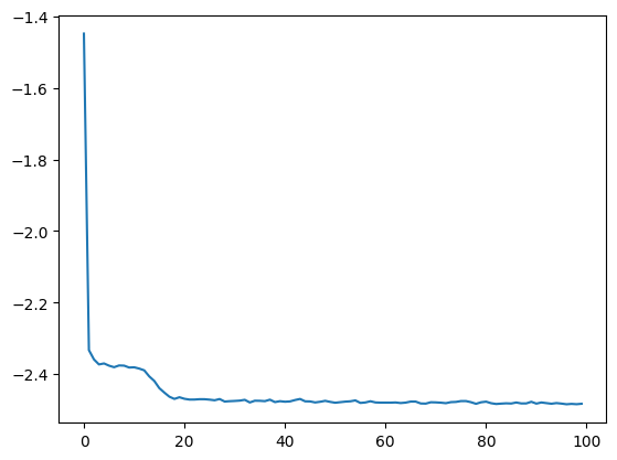
losses = dlim_regressor.fit(train_data, lr = 1e-3, nb_epoch=100, batch_size=256, emb_regularization=1e-2, save_path=model_save_path)

# Plot the loss
plt.plot(losses)
plt.show()

spectral gap = 0.9695960283279419, so we initialize phenotypes randomly
spectral gap = 0.9672122597694397, so we initialize phenotypes randomly
Model saved to ./pretrain_models/model_protein_int.pth

Visualization of the results

model = DLIM(n_variables = data.nb_val, hid_dim = 64, nb_layer = 1)

# Load pretrained DLIM model and create API instance for prediction
dlim_regressor = DLIM_API(model=model, flag_spectral=True, load_model='./pretrain_models/model_protein_int.pth')

# Predict fitness and variance for validation data
fit_v, var, _  = dlim_regressor.predict(val_data.data[:,:-1], detach=True)

# Create figure for visualization
fig, (bx, cx) = plt.subplots(2, 1, figsize=(2.3, 4))

# Calculate Pearson correlation between predicted and observed fitness
score = pearsonr(fit_v.flatten(), val_data[:, [-1]].flatten())[0]

# Predict fitness and variance for all data points
fit, var, _  = dlim_regressor.predict(data.data[:,:-1], detach=True)

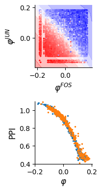
# Plot learned latent landscape for all data
dlim_regressor.plot(bx, data, xy_labels=['$\\varphi^{FOS}$', '$\\varphi^{JUN}$'])

# Remove top and right spines for cleaner plots
for el in ["top", "right"]:
    bx.spines[el].set_visible(False)
    cx.spines[el].set_visible(False)

# Replace NaN values in s1_mean with zero for plotting
df_id1["s1_mean"][np.isnan(df_id1["s1_mean"])] = 0

# Extract latent variables for each mutation
x = [dlim_regressor.model.genes_emb[0][data.substitutions_tokens[0][n]].item() for n in df_id1["id1"]]
y = [dlim_regressor.model.genes_emb[1][data.substitutions_tokens[1][n]].item() for n in df_id2["id2"]]

# Scatter plot: latent variable vs experimental mean for each protein
cx.scatter(x, df_id1["s1_mean"], label="$\\varphi_1$", s=2)
cx.scatter(y, df_id2["s2_mean"], label="$\\varphi_2$", s=2)
pearsonr(y, df_id2["s2_mean"])
pearsonr(x, df_id1["s1_mean"])

cx.set_xlabel("$\\varphi$", fontsize=12)
cx.set_ylabel("PPI", fontsize=12)
cx.set_ylim([0.4, 1.1])

plt.tight_layout()
plt.savefig("./img/lenher_2.png", dpi=300, transparent=True)
plt.show()

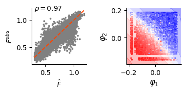
# --- Additional visualization: prediction vs observation ---
fig, (ax, bx) = plt.subplots(1, 2, figsize=(4, 2))

# Generate line for perfect prediction
x = np.linspace(min(fit_v), max(fit_v), num=100)
y = np.linspace(min(fit_v), max(fit_v), num=100)

# Scatter plot: predicted vs observed fitness for validation data
ax.scatter(fit_v, val_data.data[:, [-1]].detach(), s=3, c="grey")
ax.plot(x, y, lw=1.5, linestyle="--", c="orangered")
ax.set_xlabel("$\\hat{F}$")
ax.set_ylabel("$F^{obs}$")
# Calculate and annotate Pearson correlation on the plot
score, pval = pearsonr(fit_v.flatten(), val_data.data[:, [-1]].flatten())
ax.text(fit_v.min(), fit_v.max(), f"$\\rho={score:.2f}$")

# Plot learned latent landscape again for comparison
dlim_regressor.plot(bx, data)

for el in ["top", "right"]:
    ax.spines[el].set_visible(False)
    bx.spines[el].set_visible(False)
    cx.spines[el].set_visible(False)

plt.tight_layout()
plt.savefig("./img/lenher_2_fit.png", dpi=300, transparent=True)
plt.show()