Reproducibility 6: figure 8
Application on data from: Kinsler, Grant, Kerry Geiler-Samerotte, and Dmitri A. Petrov. “Fitness variation across subtle environmental perturbations reveals local modularity and global pleiotropy of adaptation.” Elife 9 (2020): e61271.
Import package
[ ]:
import sys
sys.path.append('../')
from dlim.model import DLIM
from dlim.dataset import Data_model
from dlim.api import DLIM_API
from scipy.stats import pearsonr, spearmanr
from sklearn.metrics import r2_score
from numpy import mean
from numpy.random import choice
import pandas as pd
from tqdm import tqdm
import matplotlib.pyplot as plt
import numpy as np
from matplotlib.patches import Patch
Subtle environment
[ ]:
# Load data from csv
infile = "../data/elife/elife_data_subtle_env.csv"
# infile = "./data/elife/elife_data_strong_env.csv"
df_data = pd.read_csv(infile, sep = '@', header = None)

data = Data_model(data=df_data, n_variables=2)

# Define the path for saving model
if infile == "./data/elife/elife_data_strong_env.csv":
    model_save_path = "./pretrain_models/model_elife_strong.pth"
else:
    model_save_path = "./pretrain_models/model_elife_subtle.pth"
Shorten the name of environment, making plot easier to show text
[3]:
colors = [
    "#1f77b4",  # Blue
    "#ff7f0e",  # Orange
    "#2ca02c",  # Green
    "#d62728",  # Red
    "#9467bd",  # Purple
    "#8c564b",  # Brown
    "#e377c2",  # Pink
    "#7f7f7f",  # Gray
    "#bcbd22",  # Olive
    "#17becf",  # Cyan
    "#aec7e8"   # Light Blue
]

# get the environments
if infile == "./data/elife/elife_data_strong_env.csv":
    ENV_LIST = ['22 hr Ferm_fitness', '1 Day_fitness', '3 Day_fitness',
                '4 Day_fitness', '5 Day_fitness', '6 Day_fitness', '7 Day_fitness',
                'Baffle, 1.8% Gluc_fitness', 'Baffle, 2.5% Gluc_fitness',
                'Baffle, 0.4 μg/ml Ben_fitness', 'Baffle, 2 μg/ml Ben_fitness',
                '0.2 M NaCl_fitness', '0.5 M NaCl_fitness', '0.2 M KCl_fitness',
                '0.5 M KCl_fitness', '8.5 μM GdA (B9)_fitness',
                '17 μM GdA_fitness', '0.5 μg/ml Flu_fitness', '1% EtOH_fitness',
                '1.5% Suc, 1% Raf_fitness']
    ENV_SHORT_LIST = ['Ferm', 'Transfer Day', 'Transfer Day',
                      'Transfer Day','Transfer Day', 'Transfer Day', 'Transfer Day',
                      'Gluc', 'Gluc',
                      'Ben', 'Ben',
                      'NaCl', 'NaCl', 'KCl',
                     # Reproducibility 5: figure 7 'KCl', '8.5 μM GdA (B9)_fitness',
                      '17 μM GdA_fitness', '0.5 μg/ml Flu_fitness', '1% EtOH_fitness',
                      '1.5% Suc, 1% Raf_fitness']
else:
    ENV_LIST = ['EC Batch 19_fitness', 'EC Batch 3_fitness', 'EC Batch 6_fitness',
                'EC Batch 13_fitness', 'EC Batch 18_fitness',
                'EC Batch 20_fitness', 'EC Batch 21_fitness',
                'EC Batch 23_fitness', 'EC 1BigBatch_fitness',
                '12 hr Ferm_fitness', '8 hr Ferm_fitness', '18 hr Ferm_fitness',
                '0.5% DMSO_fitness', '8.5 μM GdA (B1)_fitness',
                'Baffle, 1.4% Gluc_fitness', 'Baffle (B8)_fitness',
                'Baffle, 1.6% Gluc_fitness', 'Baffle, 1.7% Gluc_fitness',
                'Baffle (B9)_fitness', '1.4% Gluc_fitness', '1.8% Gluc_fitness',
                '2 μg/ml Flu_fitness', '1% Raf_fitness', '0.5% Raf_fitness',
                '1% Gly_fitness']
    ENV_SHORT_LIST = ['EC', 'EC', 'EC', 'EC',
                      'EC', 'EC', 'EC', 'EC',
                      'EC', 'Ferm', 'Ferm', 'Ferm',
                      '0.5% DMSO', '8.5 μM GdA (B1)', 'Gluc', 'Baffle',
                      'Gluc', 'Gluc', 'Baffle',
                      'Gluc', 'Gluc', '2 μg/ml Flu', 'Raf', 'Raf',
                      '1% Gly']
uni_env_short = {env: i for i, env in enumerate(list(set(ENV_SHORT_LIST)))}
conv_env = {env: env_s for env, env_s in zip(ENV_LIST, ENV_SHORT_LIST)}
inv_mut_env = {i: env for env, i in data.substitutions_tokens[1].items()}


# get the mutation types
mutation_types = ['CYR1', 'Diploid', 'Diploid + Chr11Amp', 'Diploid + Chr12Amp',
                  'Diploid + IRA1', 'Diploid + IRA2', 'Diploid_adaptive', 'ExpNeutral', 'GPB1',
                  'GPB2', 'IRA1_missense', 'IRA1_nonsense', 'IRA1_other', 'IRA2', 'KOG1',
                  'NotSequenced', 'NotSequenced_adaptive', 'PDE2', 'RAS2', 'SCH9', 'TFS1', 'TOR1',
                  'other', 'other_adaptive']

mut_type_col = {name: i for i, name in enumerate(mutation_types)}
inv_mut_type = {i: env for env, i in data.substitutions_tokens[0].items()}
[ ]:
data = Data_model(data=df_data, n_variables=2)
train_id = choice(range(data.data.shape[0]), int(data.data.shape[0]*0.8), replace=False)
test_id = [i for i in range(data.data.shape[0]) if i not in train_id]
train_data = data.subset(train_id)
test_data =  data.subset(test_id)

# Initialize DLIM model for protein interaction prediction
model = DLIM(n_variables = data.nb_val, hid_dim = 64, nb_layer = 1)
# Load pretrained DLIM model and create API instance for prediction
dlim_regressor = DLIM_API(model=model, flag_spectral=True, load_model= None)
losses = dlim_regressor.fit(train_data, test_data, lr = 1e-3, weight_decay=1e-3, nb_epoch=200, batch_size=128, emb_regularization=1e-2, save_path=model_save_path)

# Predict fitness, variance, infered phenotype for validation data
fit, var, lat  = dlim_regressor.predict(data.data[:,:-1], detach=True)
score = pearsonr(fit.flatten(), data.data[:, [-1]].flatten())[0]
print(score)
spectral gap = 0.776238203048706
spectral gap = 0.9399641156196594
Model saved to ./pretrain_models/model_elife_subtle.pth
0.9305882824966438
[ ]:
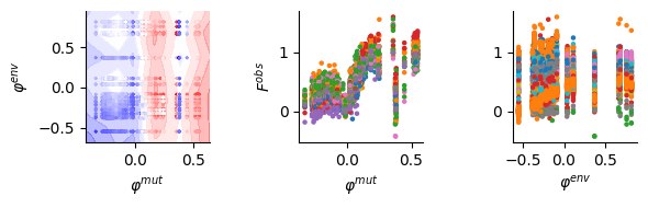
fig, (bx, cx, dx) = plt.subplots(1, 3, figsize=(6, 2))
# Original landscape
dlim_regressor.plot(bx, data, fontsize= 10)
bx.set_xlabel("$\\varphi^{mut}$")
bx.set_ylabel("$\\varphi^{env}$")

for xx in [bx, cx, dx]:
    for el in ["top", "right"]:
        xx.spines[el].set_visible(False)


dat = pd.read_csv("../data/elife/elife-61271-fig2-data1-v2.csv")
conv_bar_mut = {}
for i, row in dat.iterrows():
    if row['barcode'] not in conv_bar_mut:
        conv_bar_mut[row['barcode']] = row['mutation_type']
    else:
        assert conv_bar_mut[row['barcode']] == row['mutation_type']

# Relationship between fitness and infered phenotype
# Colored by environment
cx.scatter(lat[:, 0], data[:, -1], s=5, c=[colors[uni_env_short[conv_env[inv_mut_env[int(i)]]]] for i in data[:, 1]])
# Colored by muttaion
dx.scatter(lat[:, 1], data[:, -1], s=5, c=["C"+str(mut_type_col[conv_bar_mut[inv_mut_type[i]]]) for i in data[:, 0].int().numpy()])
cx.set_ylabel("$F^{obs}$")
cx.set_xlabel("$\\varphi^{mut}$")
dx.set_xlabel("$\\varphi^{env}$")
plt.tight_layout()
plt.savefig("./img/spec_elife_weak.png", dpi=300, transparent=True)
plt.show()
Strong environment
[ ]:
# Load data from csv for strong environment
infile = "../data/elife/elife_data_strong_env.csv"
df_data = pd.read_csv(infile, sep = '@', header = None)
data = Data_model(data=df_data, n_variables=2)
# get the environments, shorten the name
ENV_LIST = ['22 hr Ferm_fitness', '1 Day_fitness', '3 Day_fitness',
       '4 Day_fitness', '5 Day_fitness', '6 Day_fitness', '7 Day_fitness',
       'Baffle, 1.8% Gluc_fitness', 'Baffle, 2.5% Gluc_fitness',
       'Baffle, 0.4 μg/ml Ben_fitness', 'Baffle, 2 μg/ml Ben_fitness',
       '0.2 M NaCl_fitness', '0.5 M NaCl_fitness', '0.2 M KCl_fitness',
       '0.5 M KCl_fitness', '8.5 μM GdA (B9)_fitness',
       '17 μM GdA_fitness', '0.5 μg/ml Flu_fitness', '1% EtOH_fitness',
       '1.5% Suc, 1% Raf_fitness']
ENV_SHORT_LIST = ['Ferm', 'Transfer Day', 'Transfer Day',
       'Transfer Day','Transfer Day', 'Transfer Day', 'Transfer Day',
       'Gluc', 'Gluc',
       'Ben', 'Ben',
       'NaCl', 'NaCl', 'KCl',
       'KCl', '8.5 μM GdA (B9)_fitness',
       '17 μM GdA_fitness', '0.5 μg/ml Flu_fitness', '1% EtOH_fitness',
       '1.5% Suc, 1% Raf_fitness']
uni_env_short = {env: i for i, env in enumerate(list(set(ENV_SHORT_LIST)))}
conv_env = {env: env_s for env, env_s in zip(ENV_LIST, ENV_SHORT_LIST)}
inv_mut_env = {i: env for env, i in data.substitutions_tokens[1].items()}


# get the mutation types, shorten the name
mutation_types = ['CYR1', 'Diploid', 'Diploid + Chr11Amp', 'Diploid + Chr12Amp',
                  'Diploid + IRA1', 'Diploid + IRA2', 'Diploid_adaptive', 'ExpNeutral', 'GPB1',
                  'GPB2', 'IRA1_missense', 'IRA1_nonsense', 'IRA1_other', 'IRA2', 'KOG1',
                  'NotSequenced', 'NotSequenced_adaptive', 'PDE2', 'RAS2', 'SCH9', 'TFS1', 'TOR1',
                  'other', 'other_adaptive']

mutation_shorts = ['CYR1', 'Diploid', 'Diploid', 'Diploid',
                  'Diploid', 'Diploid', 'Diploid', 'other', 'GPB1',
                  'GPB2', 'IRA1', 'IRA1', 'IRA1', 'IRA2', 'other',
                  'other', 'other', 'PDE2', 'other', 'other', 'other', 'TOR1',
                  'other', 'other']
uni_mut_short = {name: i for i, name in enumerate(list(set(mutation_shorts)))}
conv_mut = {name: name_s for name, name_s in zip(mutation_types, mutation_shorts)}
inv_mut_type = {i: env for env, i in data.substitutions_tokens[0].items()}
[ ]:
if infile == "../data/elife/elife_data_strong_env.csv":
    model_save_path = "./pretrain_models/model_elife_strong.pth"
else:
    model_save_path = "./pretrain_models/model_elife_subtle.pth"

# Initialize DLIM model for protein interaction prediction
model = DLIM(n_variables = data.nb_val, hid_dim = 64, nb_layer = 1)

# Load pretrained DLIM model and create API instance for prediction
dlim_regressor = DLIM_API(model=model, flag_spectral=True, load_model= None)
losses = dlim_regressor.fit(data, lr = 1e-3, weight_decay=1e-3, nb_epoch=200, batch_size=128, emb_regularization=1e-2, save_path=model_save_path)

fit, var, lat  = dlim_regressor.predict(data.data[:,:-1], detach=True)
score = pearsonr(fit.flatten(), data.data[:, [-1]].flatten())[0]
print(score)

# Load the pretrained model
model = DLIM(n_variables = data.nb_val, hid_dim = 64, nb_layer = 1)
dlim_regressor = DLIM_API(model=model, flag_spectral=True, load_model= model_save_path)
spectral gap = 0.7917258143424988
spectral gap = 0.5240857601165771
Model saved to ./pretrain_models/model_elife_strong.pth
0.838278760208167
[ ]:
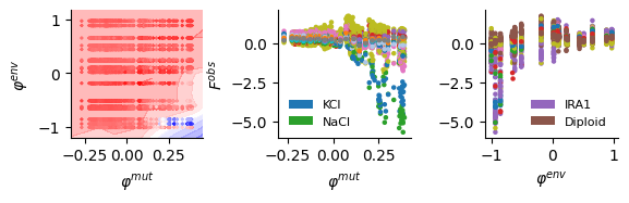
fig, (bx, cx, dx) = plt.subplots(1, 3, figsize=(6, 2))
# Original landscape
dlim_regressor.plot(bx, data, fontsize= 10)
bx.set_xlabel("$\\varphi^{mut}$")
bx.set_ylabel("$\\varphi^{env}$")

for xx in [bx, cx, dx]:
    for el in ["top", "right"]:
        xx.spines[el].set_visible(False)


dat = pd.read_csv("../data/elife/elife-61271-fig2-data1-v2.csv")
conv_bar_mut = {}
for i, row in dat.iterrows():
    if row['barcode'] not in conv_bar_mut:
        conv_bar_mut[row['barcode']] = row['mutation_type']
    else:
        assert conv_bar_mut[row['barcode']] == row['mutation_type']

# Plot the infered phenotype for mutation & enviroment vs the fitness

sel_env = ["KCl", "NaCl"]
legend_elements = [Patch(facecolor=colors[i], edgecolor='none', label=name) for name, i in uni_env_short.items() if name in sel_env]
cx.legend(handles=legend_elements, loc='lower left', fontsize=8, frameon=False)

# Colored by environment
cx.scatter(lat[:, 0], data[:, -1], s=5, c=[colors[uni_env_short[conv_env[inv_mut_env[int(i)]]]] for i in data[:, 1]])

# Colored by mutation
dx.scatter(lat[:, 1], data[:, -1], s=5, c=[colors[uni_mut_short[conv_mut[conv_bar_mut[inv_mut_type[int(i)]]]]] for i in data[:, 0]])

sel_mut = ["Diploid", "IRA1"]
legend_elements = [Patch(facecolor=colors[i], edgecolor='none', label=name) for name, i in uni_mut_short.items() if name in sel_mut]

dx.legend(handles=legend_elements, loc='lower right', fontsize=8, frameon=False)


cx.set_ylabel("$F^{obs}$")
cx.set_xlabel("$\\varphi^{mut}$")
dx.set_xlabel("$\\varphi^{env}$")
plt.tight_layout()
plt.savefig("./img/spec_elife_strong.png", dpi=300, transparent=True)
plt.show()
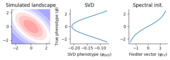
Comparison between infered phenotype from DLIM vs SVD method
[ ]:
from numpy import linspace, arange, meshgrid, array, exp, sin, concatenate, cos
from numpy import pi as npi, power, diag, allclose
from numpy.linalg import det, svd, eig
from numpy.random import normal, uniform
import numpy as np
import matplotlib.pyplot as plt

# get gaussian landscape
def rotated_gaussian_mesh(X, Y, alpha=45, center=[2.5, 2.5]):
    a = (3.14/180) * alpha
    m11 = cos(a)**2 / 2 + 2 * sin(a)**2
    m12_m21 = -sin(2*a) / 4 + sin(2*a)
    m22 = sin(a)**2 / 2 + 2 * cos(a)**2
    M = array([[m11, m12_m21],
               [m12_m21, m22]])
    det_M = det(M)
    X = X - center[0]
    Y = Y - center[0]

    F = exp(-((X**2 * M[0,0] + 2 * X * Y * M[0,1] + Y**2 * M[1,1]) / (2 * npi * det_M)))
    return F

nb_var = 40
A = linspace(-2.5, 2.5, 40)
B = linspace(-2.5, 2.5, 40)
p1, p2 = meshgrid(A, B)
land = rotated_gaussian_mesh(p1, p2, center=[0, 0])


# Use SVD to get eigen value and vectors
u, s, vh = svd(land, full_matrices=True)

recons = (u[:, :s.shape[0]] @ diag(s)) @ vh
allclose(recons, land)

fig, ax = plt.subplots(1, 3, figsize=(6, 2.2))
# Get original landscape
ax[0].contourf(p1, p2, land, cmap="bwr", alpha=0.4)
ax[0].set_title("Simulated landscape")

ax[1].plot(u[:, 0], B)
# ax[1].scatter(vh[0, :], A)
ax[1].set_title("SVD")
ax[1].set_xlabel("SVD phenotype ($\\varphi_{SVD}$)")
ax[1].set_ylabel("True phenotype ($\\phi$)")

# get similarity between mutations
def cosine_similarity_matrix(A, pearson=False):
    if pearson:
        A = A - A.mean(axis=1, keepdims=True)
    # Step 1: Compute the dot product between all pairs of rows
    dot_product = np.dot(A, A.T)  # Shape: (N, N)
    # Step 2: Compute the L2 norms of each row
    norms = np.linalg.norm(A, axis=1)  # Shape: (N,)
    # Step 3: Compute the outer product of the norms
    norm_matrix = np.outer(norms, norms)  # Shape: (N, N)
    # Step 4: Compute the cosine similarity matrix
    cosine_similarity = dot_product / norm_matrix  # Element-wise division
    return cosine_similarity + 1

pearson = True
# get similarity between mutations on gene A
A_d = cosine_similarity_matrix(land, pearson=pearson)
D_is = np.diag(1.0 / np.sqrt(A_d.sum(axis=1)))
L_aa = np.eye(A_d.shape[0]) - D_is @ A_d @ D_is

# get similarity between mutations on gene B
A_d = cosine_similarity_matrix(land.T, pearson=pearson)
D_is = np.diag(1.0 / np.sqrt(A_d.sum(axis=1)))
L_bb = np.eye(A_d.shape[0]) - D_is @ A_d @ D_is

eiv_aa, eig_aa = eig(L_aa)
eiv_bb, eig_bb = eig(L_bb)
fid_aa = (eig_aa[:, 1] - eig_aa[:, -1].mean())/eig_aa[:, -1].std()
fid_bb = (eig_bb[:, 1] - eig_bb[:, -1].mean())/eig_bb[:, -1].std()


ax[2].plot(fid_aa.flatten(), B.flatten())
# ax[2].scatter(fid_bb.flatten(), A.flatten())
ax[2].set_title("Spectral init.")
ax[2].set_xlabel("Fiedler vector ($\\varphi_{FV}$)")
# ax[2].set_ylabel("True phenotype ($\\phi$)")

for i in range(3):
    for el in ["top", "right"]:
        ax[i].spines[el].set_visible(False)

plt.tight_layout()
plt.savefig("./img/spec_laplacian_vs_svd.png", dpi=300, transparent=True)
plt.show()
[ ]: